Abusing the Instruction Cache to Store Data

Some programs use their data cache extensively, while underusing their instruction cache. We embed constant data, typically stored in memory, into the immediate fields of instructions to balance to use of both caches. We illustrate the impacts of such optimizations on the performances of a target program, describing the key parameters.

Introduction

During the Spring Semester of 2024, I, under the supervision of Prof. Clément Pit-Claudel and Alexandre Pinazza, explored the possibility of storing data in the instruction cache instead of the data cache. Before reading further, you might want to refresh your knowledge on cache hierarchy and instruction encoding. If you need more information, you can find the source code and the full report on the project's repository or send me an email at lucien.bart@alumni.epfl.ch.

To analyze the potential outcome of embedding data into instructions, we built a program spending most of its time in a tight loop. The tight loop reads a random element from two arrays, multiplies them, and adds the result to an accumulator. The randomness is achieved by filling the arrays with a permutation of their indexes. Then, we built two version of the program. In the base version, both arrays are stored in the data cache. In the optimized version, one array is stored in the instruction cache, while the other is stored in the data cache. Both versions start and end in the same way.

The base version

In the base version, the main loop is a loop summing the product of the elements.

for (int i = 0; i < nb_iter; i++)
{
    result += a[index_a] * b[index_b];
    index_a = a[index_a];
    index_b = b[index_b];
}

The optimized version

In the optimized version, we rewrite the array a as a switch-like structure. The array a is known in advance, so that we can generate the corresponding code. In c, the following switch structure

switch(index_a)
{
    case 0:
        a_value = 2;
        break;
    case 1:
        a_value = 3;
        break;
    case 2:
        a_value = 1;
        break;
    case 3:
        a_value = 4;
        break;
    case 4:
        a_value = 0;
        break;
}

is equivalent to the following array access: a_value = a[index_a]. We use the inline assembly feature of c to rewrite the array as a switch-like structure. In doing so, the code looks the following way:

retrieve_memory_address();
for (int i = 0; i < nb_iter; i++)
{
    index_b = b[index_b];
    int64_t off = index_a * 12 + 40 + memory_addr; // -O1
    __asm__ goto(
            "jmp *%[offset]\n\t"

            "mov $441, %[index]\n\t"
            "jmp %l[labend]\n\t"
            ...
            //padding from here
            "mov $484, %[index]\n\t"
            ...
            "jmp %l[labend]\n\t"
            //end of padding
            : [index] "=r"(index_a)
            : [offset] "r"(off)
            : "rax"
            : labend);
    labend:
    result += index_a * index_b;
}

The switch is coded as a jump to an address. This address depends on the value of the index. Each block is composed of two instructions, one mov and one jmp. Conceptually, it suffices to add to the current address the size of each block multiplied by the index. However, it faces two problems.

Firstly, the blocks are not all compiled to the same representation. The last few jmp are compiled to a more compact representation. To solve this issue, we add padding at the end. This way, all relevant blocks are compiled to 12 bytes.

Secondly, jumps with registers are absolute. This means that to jump to the correct position, we have to know the current address of execution, which changes at every execution of the program, due to the Address Space Layout Randomization . To retrieve the memory address, we use the following snippet.

int64_t memory_addr;
//retrieve absolute address
__asm__(
    "call next\n\t"
    "next:\n\t"
    "pop %[addr]\n\t"
    : [addr] "=r"(memory_addr)
    :);

The call instruction pushes the current address on the stack and continues the execution at the label next. Usually, the address is then poped from the stack when the execution returns from the function call. Here, we pop the stack manually and store the result in a variable. This variable is used later to calculate the destination of our custom switch case.

The last element of the offset's calculation is the value 40. This value is the difference between the place we retrieve the current address and the address where the jump occurs. This value is manually calculated and corresponds to the size of the instructions that are in between these two operations. i.e., the for loop and the access to array b.

Result

Setup

To measure the effectiveness of the optimizations, we ran experiments on an i7-8565U Intel Core computer. It is a four-core computer. Each core has one L1 data cache of 32 KiB, one L1 instruction code of 32 KiB, and one L2 cache of 1 MiB. Shared by all cores is a L3 cache of 8 MiB. Using perf, we record events occurring at the hardware level. As the behavior of the cache is nondeterministic and noisy, we run each program 30 times, unless specified otherwise. To have a clearer difference between the two versions, we set the number of iterations to 100 000 000. This way, the gain obtained by the optimization happens more times. The array b changes for each run, while the array a stays the same across all all runs.

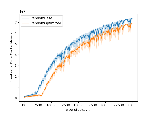
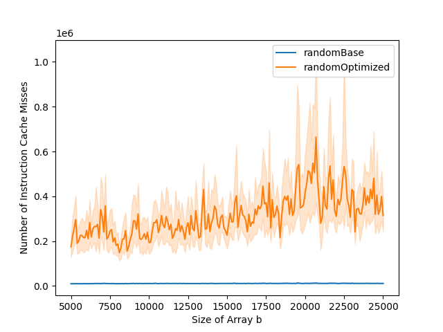
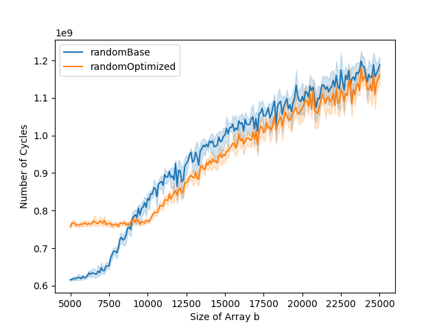
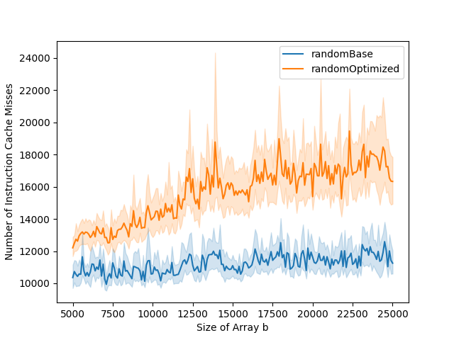
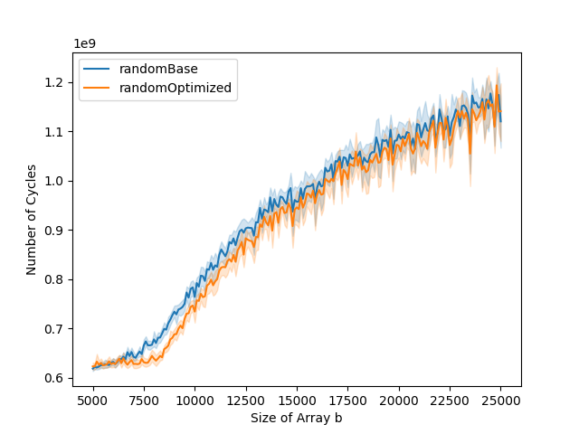
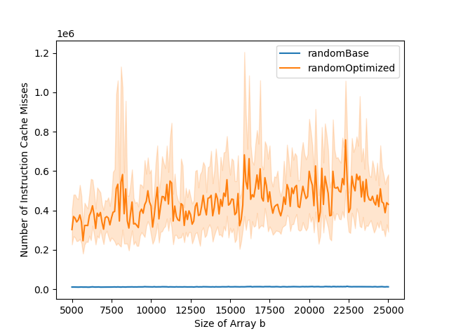
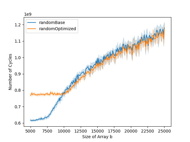
Typical Case

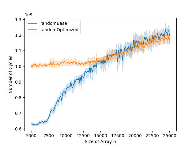
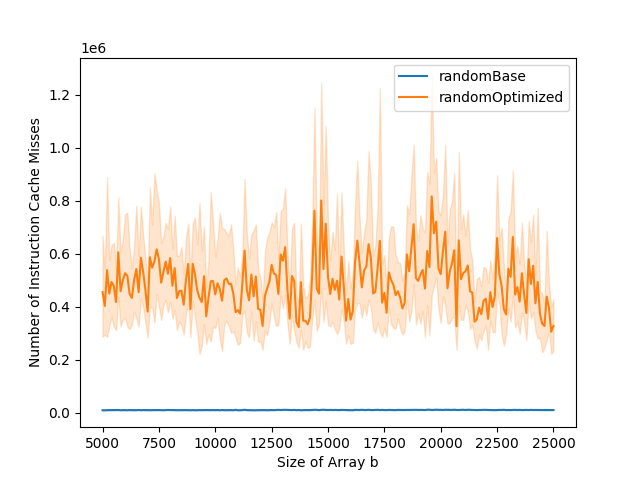
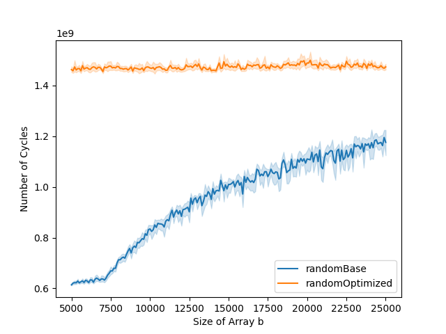
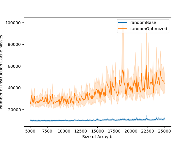
The L1 data cache misses and total number of cycles graphs can typically be divided into three parts. The first part is when both the base and the optimized versions stay stable. The second part is when only the base version starts increasing. The third part is when both base and optimized versions are increasing. In the optimized version, the number of instruction cache misses is higher than in the base version. This impacts the total number of cycles. While in the base version, the total number of cycles goes up at the same time as the number of data cache misses, this is not the case for the optimized version. This is because the bottleneck is the instruction cache misses in the first part of the graph, and it is only when the number of data cache misses gets to a certain level that it becomes the bottleneck, leading to the increase in running time.

Number of data cache misses — Illustration of the typical behavior

Number of instruction cache misses — Illustration of the typical behavior

Cycle Length

The cycle length is defined as the number of elements accessed before accessing an element that has already been accessed. It plays a crucial role in the execution time.

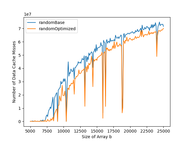
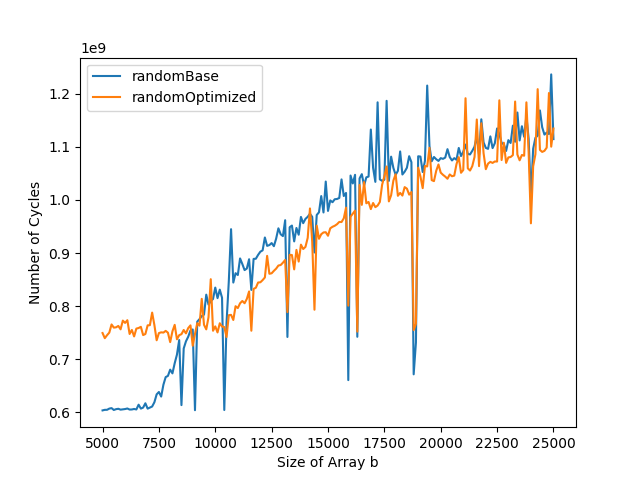
On b

By running the program only once, we can analyze the impact of the varying cycle length of b. In the total number of cycles and data cache misses graphs, we can observe dips. These dips are due to very short cycles for b. When the cycle length is small, only a few elements are accessed. Thus, it does not fill the cache.

Running time — Impact of small cycle length

On a

To analyze the impact of the cycle length of a, we set a fixed size for a but with varying cycle lengths. In the graphs, we observe that the bigger the cycle length, the slower the optimized version for small b, in the first part of the graphs. When the cycle gets too big, the optimization is not worth it anymore. A possible explanation is as the cycle length is bigger, more code is accessed, leading to more instruction cache misses.

Change of size of array a

The previous explanation however doesn't stand for the following example. In this example, we keep a similar cycle length but the size of a varies. While the number of instruction cache misses increases with the size of the array, the running time stays similar. The increase in instruction cache miss can be explained by the fact that caches operate in blocks and that more useless code is fetched into the instruction cache when the array is bigger, as the cycle is more sparse in the array.

Number of instruction cache misses for cycle 496 and size 500 — Comparison of similar cycle lengths (~500) but with different sizes of array a

Number of cycles for cycle 496 and size 500 — Comparison of similar cycle lengths (~500) but with different sizes of array a

Ideal situation

We can obtain an optimal situation by adjusting both the size of a and its cycle length. On the test computer, the ideal cycle length is 500. When bigger, the optimization is not worth it and when smaller, it doesn't offer a lot of benefits. Increasing the size of array a shifts the moment when the running time of the base version starts to grow significantly while staying the same for the optimized version. This leads to results of around 10-15% increases for the array size of a being 2000 and the cycle length 500.

Conclusion

In our project, we have shown how to embed constant data typically stored in memory in immediate fields of instructions. We have illustrated the impacts of such optimizations on the performance of a program, emphasizing which parameters are of particular interest. It would be beneficial to understand more deeply the relationship between the instruction cache misses and the running time. A possible extension to the project is to generate the code for the optimization using some form of JIT compilation and look for real programs that would benefit from this optimization.